Computer Vision - Using the MV1 to Automatically Measure Plants

@ajc3xc


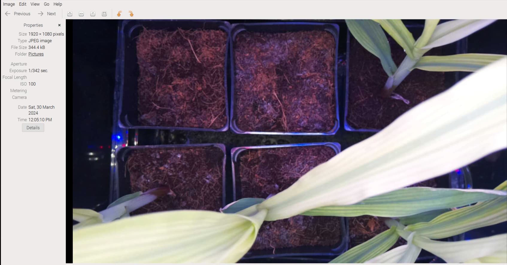
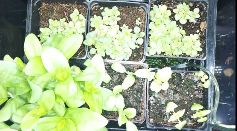
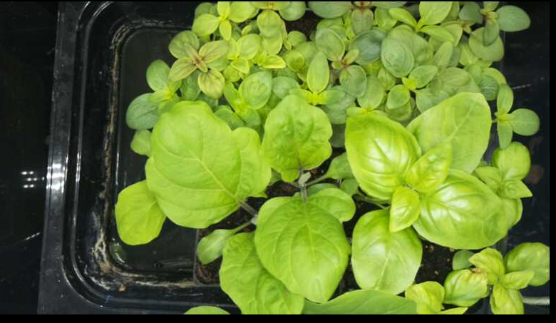
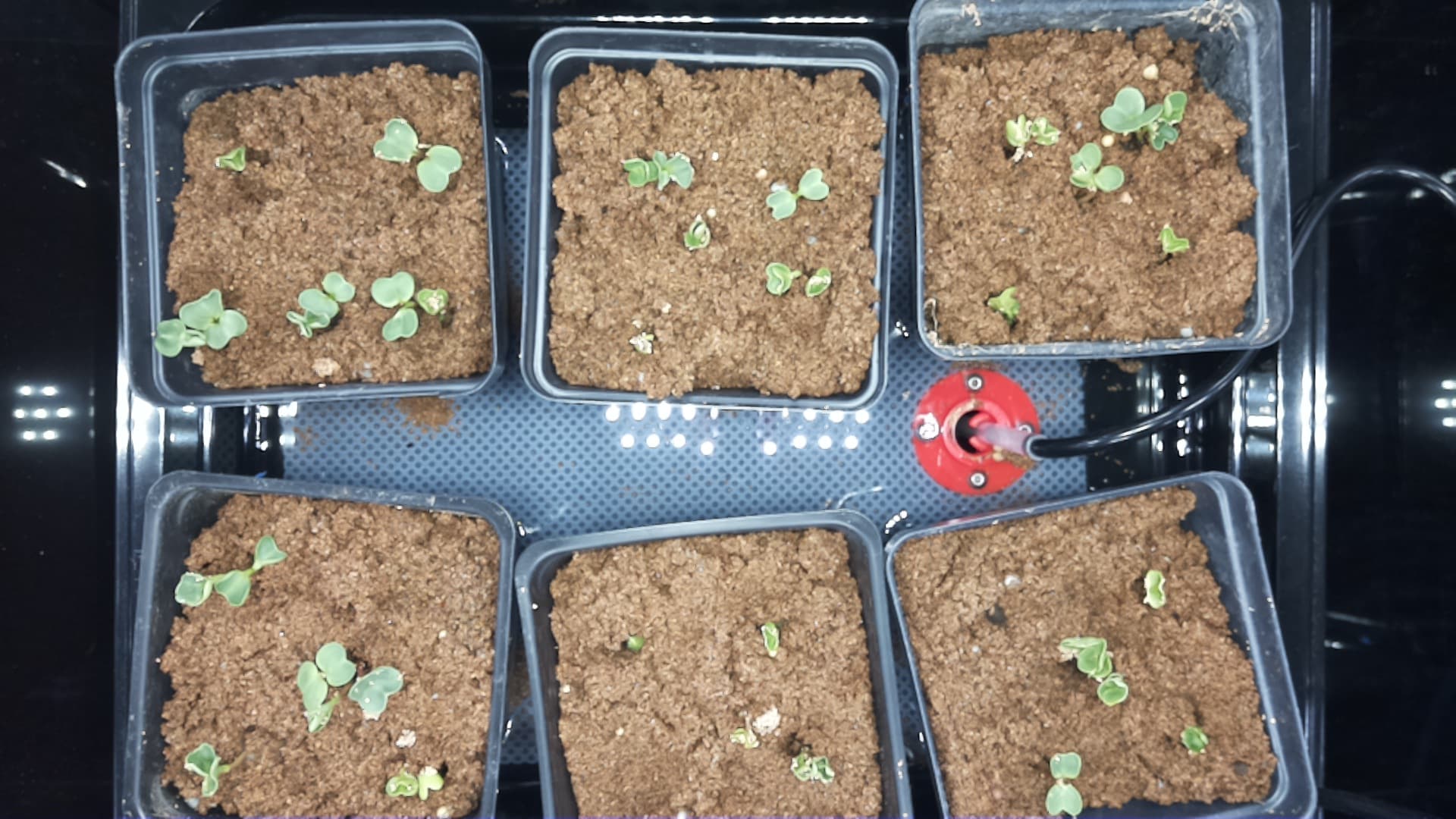
If you have PlantCV installed, it installs OpenCV as well, so the following code should work in your environment. Either use the attached file, or an image of your choice.

This is the file Find_Plant.py - the main file:

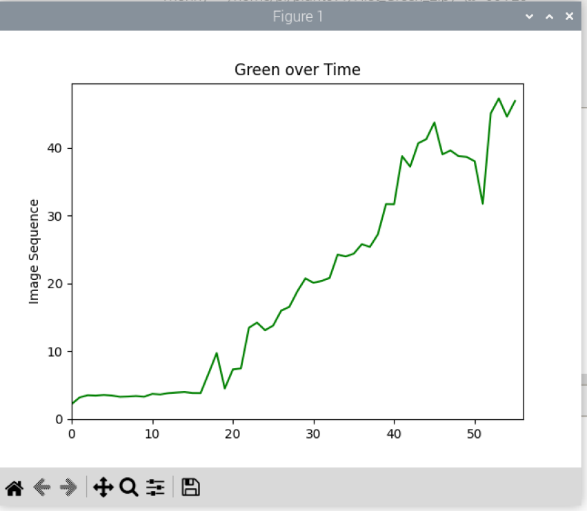
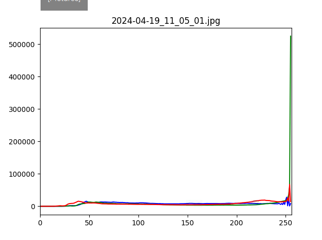
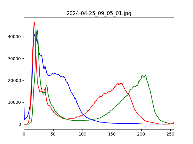
Test code working on a un-warped single image

import numpy as np
import cv2
import PlantUtil as fpu

# 

v2.imread(pic)
#warp=fpu.transform(src, pts_in, pts_out)
#cv2.imshow('Warp', warp)

mask=fpu.getMask(src, lower, upper)
cv2.imshow('Mask',mask)
cv2.waitKey(2)

#res = cv2.bitwise_and(warp,warp, mask= mask)

edge=fpu.getEdges(mask)
cv2.imshow('Edges', edge)
cv2.waitKey(2)

ellipse=fpu.getContours(edge, src)
print(type(ellipse))

cv2.imshow('Elipse', ellipse)
#cv2.imwrite('/home/pi/MVP/Pictures/Ellipse.png', src2)

# Wat for the escape key to be pressed to end - does not work with Python IDE
k = cv2.waitKey(0) & 0xFF
cv2.destroyAllWindows()

PlantUtil.py are the utility functions that do the work:


# Routines to find plants and draw ellipse

import numpy as np
import cv2
import copy

def transform(src, pts_in, pts_out):

    # Prepare the image for work, straighten and clip
    #gimg=cv2.imread(pic, cv2.IMREAD_GRAYSCALE)
    # Perform transformation warp
    M=cv2.getPerspectiveTransform(pts_in, pts_out)
    #print(M)
    warp=cv2.warpPerspective(src, M,(724,720))
    return warp

def getMask(img, lower, upper):
    
    wh, bk, mask = get_pixels(img, upper, lower)

    # erode and dialate the image to remove artifacts
    kernel = np.ones((5,5), np.uint8)
    erosion = cv2.erode(mask, kernel, iterations = 1)
    dilation = cv2.dilate(erosion, kernel, iterations=5)
    erosion2 = cv2.erode(dilation, kernel, iterations = 3)

    # Create a test image showing the green through the mask
    # Not actually used, but interesting to play with
    return erosion2

#bgr=cv2.cvtColor(erosion2, cv2.COLOR_HSV2BGR)
#gr=cv2.cvtColor(res, cv2.COLOR_BGR2GRAY)

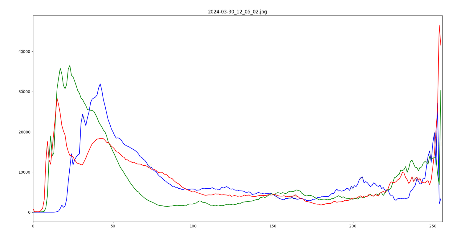
def get_pixels(img, upper, lower):
    #Begin finding of plants
    # Convert BGR to HSV
    hsv = cv2.cvtColor(img, cv2.COLOR_BGR2HSV)

    #print("image type: ", type(hsv))

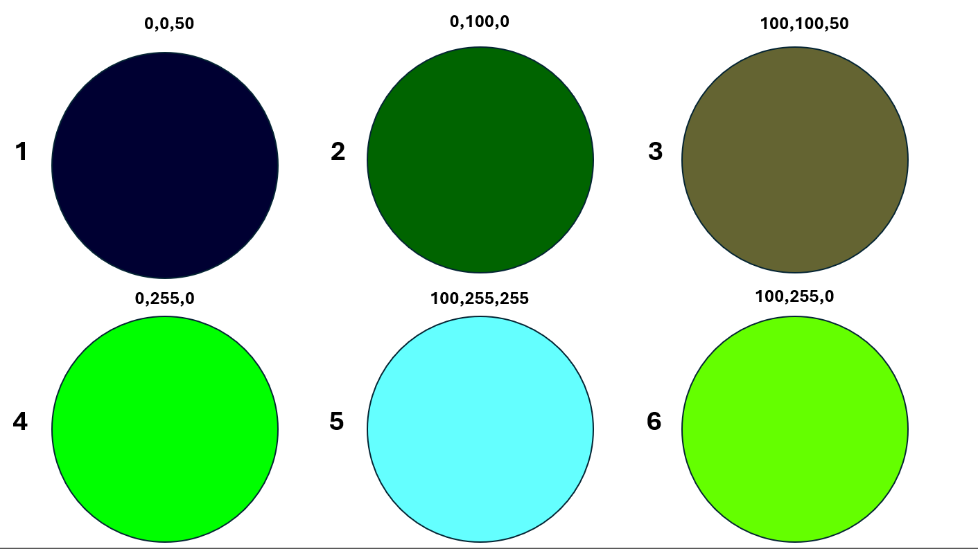
    # Threshold the HSV image to get only green colors and create mask of greens
    mask = cv2.inRange(hsv, lower, upper)
    height, width =  mask.shape[:2]
    wh = np.sum(mask == 255)
    bk = np.sum(mask == 0)
    sz = wh + bk
    
    return wh, bk, mask
    #print(f'Size: {height * width}')
    #print(f'Mask Size: {sz}')
    print(f'White: {wh}')
    print(f'Black: {bk}')
    print(f'Ratio: {round(wh/sz, 2)}')
    

def getEdges(img):

    BLACK=[0, 0, 0]
    #Border the image so edges run around ends
    bdr=cv2.copyMakeBorder(img, 10, 10, 10, 10, cv2.BORDER_CONSTANT, value=BLACK)

    # Detect the edges of the plants
    edges=cv2.Canny(bdr, 100, 200)
    print(edges.shape)
    return edges

def getContours(img, display):
    # Build contours of the plants from the edges
    # Only get top level (external) contours
    contours,hierarchy= cv2.findContours(img, cv2.RETR_EXTERNAL, cv2.CHAIN_APPROX_SIMPLE)
    # Copy the image, otherwise it would be overwritten and no longer available
    out=copy.copy(display)
    # Walk all the contours
    x=0 # Counter for display
    for i in contours:
        x=x+1
        # Create and draw the elipses - this is the final output image
        if cv2.contourArea(i) > 5:
            ellipse = cv2.fitEllipse(i)
            cv2.ellipse(out, ellipse,(0,0,0),2)
        else:
            print("Too small of area for evaluation", x, cv2.contourArea(i))
        
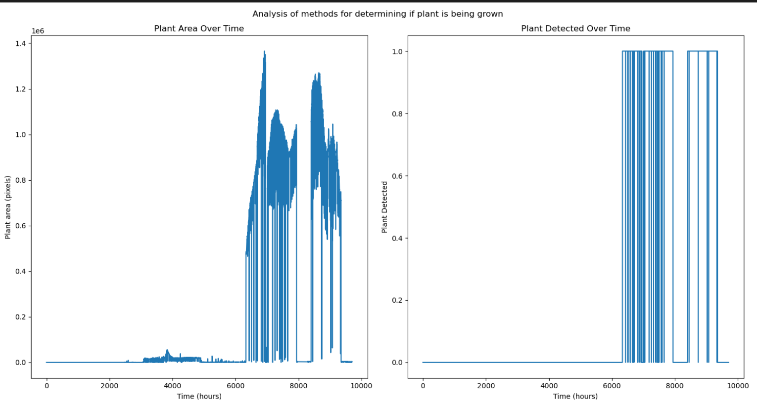
        # The area could be used to calculate phenotype info
#        print("Contour: ", x, "Area: ", cv2.contourArea(i))
    return out
''''
1 Like

@hmw
Thank for sharing. Looking at your code and comparing it to the workflow I’ve used for plantcv, it seems like erosion has a similar function to plantcv’s fill in that it removes small background noise, and dilate to fill_holes in that of the dilate function and the ellipse to plantcv’s roi function. This could certainly be useful later down the line when trying to do things with regions of interest and more in depth processing of the plants in a dataset.

@Peter
Here is a script I’ve been working on for a bit over a day trying to test a method for step 1.

I’m getting times of about 20-30 seconds for the ~1400 images for the dataset provided. I tested out various other methods (dask, swifter, mapply, pyspark), and they either didn’t work (dask, swifter), or were slower (mapply, pyspark).

For the output of the files, would you like me to store them on a seperate folder of the boto3, or do you want me to create a list file of the images I would be using as the dataset?

I was able to get boto3 working, so I have access to the entire marsfarm dataset. I just did some experimentation with traversing the folder structure of the s3 buckets. Do you know which buckets correpspond to which experiments (i.e. regini labs, summer 2023 and summer 2024)?

Looking back over the code I made for checking for seedlings / plants, I removed some unnecessary code and reduced the time to about 12-18 seconds, so almost twice as fast. I still need to figure out how to get the code to work on pyspark, since we are dealing with very large amounts of data and not even 64 cores and a slimmed down algorithm will make a difference. Compared to the single core setup it’s like a micro car to a pickup truck, but what we need is a dump truck.

For now I’m going to test the algorithm on one of the devices in either the regini or production bucket that have trials with empty / unplanted boxes, to work on getting step 1 ready.

For step 2, I’m going to use the pre-existing dataset from google drive for this. I’ll have to do more research on pre-existing plant identification algorithms out there, whether that be neural networks or some other traditional ml algorithm. I’ll also have to look at how the OpenAI vision model analyses the plants.

As for step 3, hopefully I can get the other 2 steps done quickly and look at that part within a few weeks to a month.

Finally, do you want me to directly edit the metadata for each of the photos in s3, or do you want me to say save a copy in a different bucket first for testing before we do the entirety of s3? I’m still trying to get a grip on how s3 works, so in the meantime it would be best not to permanently alter enormous amounts of data.

I’ve been continuing to test out applying my function to the s3 bucket. Currently, I’m researching how to add has_plant as an attribute to each of the jpg images, but I’m not sure where the metadata / measurements for each of the images is located. I see that the heroku app has temperature, humidity, and co2, but I’m not sure where that is located, and if so how to add a new field called ‘plant_area’.

Testing out my algorithm on the images in s3, it seems to significantly struggle with false positives. There’s an example here in this notebook that demonstrates it pretty clearly.

I think I have a solution, but I am working from a different direction (checking the images at the time they are taken). I am then loading the results into my database to use my existing charting. This is in prototyping, but might give you some ideas. Images can come from anywhere, and this can be modified for batch processing.
First the cheats:

  1. Cover each pot (I have six) with a 3.25x3.25 yellow card and get an image. This will tell you 1) the area covered by each card (ie pixels to cm2), and let you crop out each pot for individual processing.
    a) Create a mask (using upper and lower yellow color ranges)
    b) Find the edges (Border and Canny edge detection)
    c) Get contours and create bounding boxes - there should be six
    d) save the dimensions as an array of arrays to a file (roi.py)
  2. For each picture.
    a) crop the pots from the image into sub images (simple numpy array sub-setting)
    b) for each pot, get a pixel count of the pixels between a high and low HSV value
    c) divide the pixels by the above determined pixel/cm ration for the area that is a plant. If it is 0, the plant has not germinated yet.

I need to get the code into GitHub so it can be shared

This is a good example of a hardware requirement for the MV1 that is not flexible to us as developers. We don’t plan to add a second camera, NIIR cameras, or adjustable height features anytime soon. I’m worried that we’re jumping to the ‘cheats’ (which rely upon changes to the hardware) before fully understanding the requirements and the nature of the platform. Just as one quick example, here’s another thing to consider about our dataset being timeseries:

They will always be sequential - this is a timeseries dataset. Depending on our rate of capture (currently once an hour, but could be more if there was a use case) we can easily reference an image that should be very similar to the one being taken.

I’m concerned about your approach @hmw not being applicable to anything beyond one set of images. Assuming step 1 is completed correctly, using cards to identify the ROI, wouldn’t any movement of the reservoir itself throw that ‘calibration’ off?

In a school environment, students will inevitably be removing the reservoir to fill it with water, at which time they may also remove the pots to measure them or thin them as well. I would like for any solution to be able to work for MV1 users with 3" pots but also using 2" net cups, net pots, or hydroton balls as well. Unless we first explore that route and determine it to be impossible - I’d like to maintain that goal. Photos in this thread are good examples: MV1 Summer Trials

I know this is not the same as an algorithm to accurately measure plants. That’s not what we want. We want to know if Suzies tomato plant is dying (getting smaller) or if Billies radishes have germinated (any green dots) yet - that’s it.

I would be curious for someone on @ajc3xc’s team to read this paper titled ‘Segmentation of Overlapping Plants in Multi-plant Image Time Series’ by Dr. Malia Gehan at Danforth.

@Peter @ajc3xc
As the cover to “The Hitchiker’s Guide to the Universe” says, “Don’t Panic”
I am doing R&D looking toward the future and trying to solve a pot level (individual plant) issue, and identifying the barriers that need to be addressed for getting germination and plant growth up until the plants start spreading into each other…
Peter is working on a historical administrative problem of of which boxes got used, and how well did they do generally.
Getting the ROI (region of interest) is a difficult problem for historical images, but if you are only interested in if ANYTHING was growing, then it is easy to identify the whole image as a single ROI. I have also separated my ‘engine’ from the ‘feeder’, so you could have code to walk the entire S3 (hopefully chunking it into separate trials) and pass it to the engine.
I am assuming @ajc3xc has the feeder for S3 working, and he can either modify what I have, or just as easily re-write it. The only critical work is:
# mask the green pixels in the image
green_mask = cv2.inRange(img, lower, upper)
# count the white pixels in the mask
return np.sum(green_mask)

Then save the data out somewhere for reporting or charting. You may be more interested in the slope of the data than the actual counts. Even if the range is off, if there is no increasing slope over time, there is probably nothing growing.

If you want to go deeper, you can always try and identify contours in the green_mask, ideally there is one contour per plant:
contours, hierarchy = cv2.findContours(green_mask, cv2.RETR_EXTERNAL, cv2.CHAIN_APPROX_SIMPLE)

I found this program (with minor modifications) great for getting mask color ranges. Take a sampling of test images and see if you can get a consistent hit on a green range. For your administrative needs, it probably doesn’t need to be too accurate.

1 Like

@Peter @ajc3xc
I am making a pivot. The color ranges (UPPER & LOWER) were giving problems when the color was not stable. So, switched from inRange to using calcHist.
Histogram uses RGB, so a lot of colors are a mixture of the three - but plants contain pure green (value=255), which should not be in the rest of the image.
I filtered out low values (bad images that are all black), keeping only those with over 2000 pixels, as this gives a good plot. This is simple code, but gives a good relative evaluation.
Again, it should be easy to swap out my file feeder with a database feeder. Group images by trial and sort by date. You can set a threshold on the trial, anything below the threshold should be consider devoid of plants.
The following chart is my current trial (not complete), using hourly images.

Code:

import numpy as np
import cv2 as cv
from matplotlib import pyplot as plt
import os

Location of images

DIR = ‘/home/pi/plantcv1/Pictures/’

Test images

pic = ‘2024-03-15_21_21_08.jpg’ # no plant
#pic = ‘2024-03-17_18_48_14.jpg’ # seedlings
#pic = ‘2024-03-22_10_05_01.jpg’ # plant

CONST = 2000 # pixels per sq cm, calculated previously

class Measure_Green(object):

def main(self):
    # holder for key statistic
    cnt = []
    files = self.get_files()
    for file in files:
        # process each file, get count of green from RGB array
        histr = self.measure(file)
        # strip out green 
        nbr = histr[255]
        #print(nbr)
        # Filter for no values and strays
        if nbr > 2000:
            cnt.append(nbr/CONST)
    
    self.show(np.array(cnt))        

def get_files(self):
    # get sorted list of files from directory
    files = []
    list = sorted(os.listdir(DIR))
    for file in list:
        if '2024' in file:
            # only get images (datetime label)
            files.append(file)
    #print(len(self.files))
    #print(self.files)
    return files
            

def measure(self, file):
    # open image and get histogram
    #print(file)
    img = cv.imread(DIR+file)
    assert img is not None, "file could not be read, check with os.path.exists()"
    
    # not used, used for plotting all color chanels
    color = ('b','g','r')
    # get just green chanel (ie 1); 255 buckets, range 0-256
    histr = cv.calcHist([img],[1],None,[256],[0,256])
    return histr

def show(self, histr):
    # plot display
    #print(histr)
    plt.plot(histr,color = 'g')
    plt.xlim([0,len(histr)])
    plt.ylabel('Sq CM')
    plt.ylabel('Image Sequence')
    plt.title('Green over Time')
    plt.show()

def test():
mg = Measure_Green()
mg.main()

if name==“main”:
test()
print(“Done”)

1 Like

@Peter @ajc3xc
I need to clean up the page, but the data and query are working at the plot level:


Plants are big enough now that they are covering more than one pot/plot area, so not accurate in the detail.
Need to see what can do walking the trials in S3.

1 Like

This is it - I didn’t know what I wanted exactly until seeing it but here it is!

@ajc3xc these are your next steps.

Could you please elaborate on the difference between inRange and calcHist? Also, is there a reason you’re so confident that all plants will contain true green - I just want to understand if that’s indeed a ‘fact’ and what has told you that. From what I understand, you’re saying that you look for images with more than 2000 pixels match ‘pure green’ (255 in the RGB scale). Can you help me understand by explaining how each of the six circles below (think of them as pixels), each with a unique RGB code, would be counted? I can see in your code where you’re selecting only the green pixels, so I assume it would count 5 of the 6 circles shown below - is that correct? Does this mean that if there were a big blue piece of paper in the box would all of those pixels be counted as a ‘plant’ too?

We are certainly interested in the slope. Slope is what could tell me for sure whether it’s a plant - because blue pieces of paper don’t increase in size every hour. On that note, I’m curious to know what happened to the plants in your box at this time - is that accurate? Did they wilt or something?
image

The easiest way to understand the color is to run the following program. Set green to max then play with the others. Drop the green and you don’t get much green.
Program thanks to ChatGPT:

import matplotlib.pyplot as plt
from matplotlib.widgets import Slider

Initial RGB values

initial_rgb = [0.5, 0.5, 0.5]

Create a figure and an axes

fig, ax = plt.subplots()
plt.subplots_adjust(left=0.25, bottom=0.25)

Remove axes for cleaner look

ax.set_xticks()
ax.set_yticks()

Create a rectangle that will display the color

rect = plt.Rectangle((0, 0), 1, 1, color=initial_rgb)
ax.add_patch(rect)

Adjust the main plot to make room for the sliders

plt.axis([0, 1, 0, 1])

Create axes for sliders and then sliders

axcolor = ‘lightgoldenrodyellow’
ax_r = plt.axes([0.25, 0.1, 0.65, 0.03], facecolor=axcolor)
ax_g = plt.axes([0.25, 0.15, 0.65, 0.03], facecolor=axcolor)
ax_b = plt.axes([0.25, 0.2, 0.65, 0.03], facecolor=axcolor)

sld_r = Slider(ax_r, ‘R’, 0, 1, valinit=initial_rgb[0])
sld_g = Slider(ax_g, ‘G’, 0, 1, valinit=initial_rgb[1])
sld_b = Slider(ax_b, ‘B’, 0, 1, valinit=initial_rgb[2])

Update color function

def update(val):
rect.set_color((sld_r.val, sld_g.val, sld_b.val))
fig.canvas.draw_idle()

Call update function on slider value change

sld_r.on_changed(update)
sld_g.on_changed(update)
sld_b.on_changed(update)

plt.show()

1 Like

FYI:
The drop in green in the chart is due to lighting issues. I filter out any files where the number of green pixels is below 2000 (night when the light didn’t come on), but this was where the image was very dark (but not all black).

1 Like

this would be great as a ‘stacked area’ chart - that would show the cumulative total amount of green pixels with its best guess as which plot those are attributed to.

My charting of plant growth took an unexpected turn, with the values dropping off as the plants are getting bigger.


(Plot of green[255] from start of trial to present, one line per pot/plot)

Looking at the image, and the full spectrum histogram explains things:


(Recent image from the MV)

(RGB Histogram of the plant image)

The plant is not bright green, but white with green stripes, and the closer to the light it gets the more bleached the photo looks.
This is evident in the histogram, as the right shows a green spike, but blended with other colors. The colors on the left are the soil and other parts of the box - they are consistent in most of the images.
My conclusion is that while looking for the green channel for bin 255 works as a general indicator of plants being present, and catches early stage growth, you have to understand the plants, lighting and camera to correctly interpret the data. to get the full life cycle growth will still require more complicated processing, that may end up being species specific.

@Peter
I needed to make a change to the camera software:
rpicam-still -t 5000 --nopreview --gain 1.75 --shutter 10000 --width 1920 --height 1080 -o {}'.format(IMAGE_DIR + file_name

This gives a fixed shutter time (1/100) and iso (175). This avoids the ‘red’ images where the iso drops to 115. The ‘red’ images are noticeable in the graph, as these are the low spikes. This image is where one pot of seedlings has germinated and the others have not started.

@Peter
Dynamic systems are a pain. Progress in one area often leads to disruptions in what seemed stable.
I was charting histograms to show plant growth, getting the ‘bin’ for 255. This worked great, until I made some adjustments to the lights and camera - then the histogram shifted. The images had been a bit over exposed, but gave a good reading at 255
2024-04-19-11-Hist
Plotted over the trial of just the histogram X axis 255 bin. Note the loss of the trendline toward the end of the graph when the lighting was changed.
Field_255

The following is after the change to the camera and lighting:

There had been a timing problem between the normal light setting and the camera light setting (ie the downward spikes in the graph). However when this got fixed, I lost the 255 bin. The images are better (not over-exposed) but it shifted the histogram.
2024-04-25-09-Hist
The following chart is the sum of the bins >= 150 (histogram chart X axis)
150


Field_150
Definitely fixed the lighting issues, but this introduced new problems. The charts tell a good story (evidence of the lighting issue, which stops toward the end of the graph; the removal of two pots [drop in trend]). Just wish I could find a way to consistently get the charting without having to re-adjust for every light condition and variation.

To try and narrow down the candidates for plant image processing to develop a good phenotypical model, I implemented a mask that uses a combined hsv and lab masks to better seperate out the images. After doing some testing to make sure that the mask performed well on the small sample dataset I had, I ran it on the entire mv1 production bucket.

I used an estimate of > 100k for whether or not a plant is in the bucket, and I made an algorithm deciding to tag all the images in a prefix as ‘mayhaveplant’: 1 if any image in the folder was > 100k, and ‘mayhaveplant’: 0 if there was no images > 100k in the folder. Here are some example plots. They are a bit messy, and I would probably need to examine the images in futher detail to see what is going on.

Here is a link to the full results I generated in the mv1-production bucket as of 4/29/2024

ok, so I am just now looking at this post and this is super cool!

1 Like

After having finished the capstone project for this semester, I developed lambda code that would be applicable to be usable to apply to all of the s3 objects. I replaced the plantcv functions I used with skimage for speed, but I haven’t tested them yet to ensure they work. The session credentials probably wouldn’t be needed in lambda, so adjust that as needed.

Here is the code:

#!/usr/bin/env python3
import boto3
from botocore.client import Config as BotoConfig
from botocore.exceptions import ClientError, ResponseStreamingError
import numpy as np
import cv2
from copy import deepcopy
import configparser
from PIL import Image, UnidentifiedImageError, ImageFile
ImageFile.LOAD_TRUNCATED_IMAGES = True
from io import BytesIO
from skimage import morphology
from skimage.measure import label

#doctor, are you sure this work?
#haha, I have no idea!
import urllib3
urllib3.disable_warnings(urllib3.exceptions.InsecureRequestWarning)

# Create a ConfigParser object
config = configparser.ConfigParser()

# Read in access key and secret key
config.read('/mnt/stor/ceph/csb/marsfarm/projects/aws_key/aws_key.cfg')

# Accessing the values
# Access a specific section
settings = config['Secrets']

#DO NOT PRINT secret access key or key id
session = boto3.Session(
    aws_access_key_id=settings['aws_access_key_id'],
    aws_secret_access_key=settings['aws_secret_access_key'],
)
config = BotoConfig(connect_timeout=120, read_timeout=300, retries={"max_attempts": 5, "mode": "standard"})
s3 = session.client('s3', config=config, verify=False)

def lambda_return(plant_pixels, MayHavePlant, number_of_plants):
    return {
        'statusCode': 200,
        'body': {
            'estimated_plant_area': plant_pixels,
            'MayHavePlant': MayHavePlant,
            'estimated_number_of_plants': number_of_plants
        }
    }  

def lambda_handler(event, context):
    bucket_name = event['bucket']
    key = event['key']

    # Retrieve image from S3
    try:
        response = s3.get_object(Bucket=bucket_name, Key=key)
        image_content = response['Body'].read()

        # Open the image using PIL
        #not using chunks, assuming it doesn't fail
        image = Image.open(BytesIO(image_content))
    except UnidentifiedImageError as e:
        print(f"{key} won't load")
        return lambda_return(0, 0, 0)
    except urllib3.exceptions.SSLError:
        print(f"SSL failed for {key}")
        return lambda_return(0, 0, 0)
    except ResponseStreamingError as e:
        print(f"ResponseStreamingError for {key}")
        return lambda_return(0, 0, 0)
    
    #convert to 3d numpy array
    image_np = np.array(image)
    
    # Convert to HSV and LAB color spaces
    hsv_image = cv2.cvtColor(image_np, cv2.COLOR_BGR2HSV)
    lab_image = cv2.cvtColor(image_np, cv2.COLOR_BGR2LAB)

    # Define HSV range for filtering using OpenCV
    # OpenCV uses 0-180 for Hue, so the values are halved
    hsv_min = np.array([int(28/2), int(20/100*255), int(20/100*255)])
    hsv_max = np.array([int(144/2), 255, 255])
    hsv_mask = cv2.inRange(hsv_image, hsv_min, hsv_max)

    # Define LAB range for filtering using OpenCV
    # OpenCV uses 0-255 for L, a*, and b*
    # Note: 'a' and 'b' ranges need to be shifted from [-128, 127] to [0, 255]
    # L is scaled from [0, 100] in LAB to [0, 255] in OpenCV
    lab_lower = np.array([int(10/100*255), 0, 132])
    lab_upper = np.array([int(90/100*255), 124, 255])
    lab_mask = cv2.inRange(lab_image, lab_lower, lab_upper)

    # Combine the masks (logical AND) and apply to the original image
    combined_mask = cv2.bitwise_and(hsv_mask, lab_mask)
    
    #remove small objects in the image so object detection won't be as bad
    denoised_mask = morphology.remove_small_objects(combined_mask, 500)

    #output mask to file
    #denoised_filename = image_folder / ("denoised_mask_" + Path(key).name)
    #if not denoised_filename.is_file(): cv2.imwrite(str(denoised_filename), denoised_mask)

    #count the number of nonzero pixels, determine if > 110k
    plant_pixels = cv2.countNonZero(denoised_mask)
    MayHavePlant = bool(plant_pixels > 110000)

    #create labels for masks that may have plants, count number of objects
    number_of_plants = 0
    if MayHavePlant:
        # Label connected regions
        labeled_mask = label(denoised_mask, connectivity=1)  # You can adjust connectivity (1 or 2)

        # Find the number of objects by ignoring the background (label 0)
        number_of_plants = len(np.unique(labeled_mask)) - 1  # Subtract one for the background label

    # Here, you might want to save or further process the result_image
    # For demonstration, let's just return the number of white pixels in the mask
    lambda_return(plant_pixels, MayHavePlant, number_of_plants)
    return plant_pixels, MayHavePlant, number_of_plants

Output of this code in post #59 by [ajc3xc]

Notes from call w/Adam this afternoon

s3 metadata

  • ‘estimated_plant_area’
    • estimated area of plant from non-zero pixels > this goes beyond just ‘looking for green pixels and also uses several layers of masking that were found to be effective based on testing of images taken in MV1s’
    • filter for hue, separation and value as one mask > likeness
    • uses RGB, and then also converts to HSV
    • uses a mathematical extrapolation to create an array of values known as the ‘mask’
  • ‘MayHavePlant’
    • yes/no value based on evaluation of whether there are more than 110k pixels in the mask. This number was picked because it was found to be a likely determination of there actually being a plant in that photo.
    • known bugs/limitations: sometimes there can been small plants that go undetected.
  • ‘estimated_number_of_plants’
    • known failures/bugs/limitations: when algae accumulates in the media or wicking mat. The masking method is not able to be rendered as an annotated image
    • reasons we went this way: to differentiate plants as they grow older and overlap, a unique identity and location for that plant would need to be maintained throughout the trial.

Next steps

@ajc3xc will test this exact version of the code (just comment out lambda section) on 10 different images of plants.

  • Bok Choy (7 days, 14 days, 21 days)
  • Lettuce (7 days, 14 days, 21 days)
  • Radishes (7 days, 14 days, 21 days)
  • Basil (7 days, 14 days, 21 days)
  • Tomatoes (7 days, 14 days, 21 days)

Notes from 05/05 meeting with @Holden and @ajc3xc

Useful outcomes from their project for MARSfarm

  1. @Holden create a higher fidelity user interface for teachers and students to ‘analyze’ a photo using computer vision I belive he has started work on translating his paper sketches into a drafted user interface using Canva. We’ll be sure to share the results here when he’s finished!
  2. @ajc3xc > Convert his work on labelling images in MV1 S3 buckets into an AWS lamba function so that it can be integrated into MARSfarm’s production services.
    a. convert the ‘has plant in it’ function into a lambda script - I think this is already done
    b. convert function for ‘create labels’ that will create the estimated number of seedlings I think this is also already done - at least we’ll have a ballpark of accuracy based on the test results Adam will share
    c. function to take one photo and return two photos: one masked, one with regions of interest annotated, and also charts of RGB distribution. This could also be an effort to package up some of what we’ve observed to ‘work’ with regards to successfully annotating images.

@hmw please also feel free to contribute suggestions for use cases based on the code that you’ve known to work well. @ajc3xc is going to keep working with us over the summer (as much as his other jobs allow) on this project so if you have suggestions for how to improve the masking process he outlines in his code - I’d appreciate it. I trust you guys here to be the experts - I just understand you make pictures turn into numbers and then do math with that.